In the first post of this three-part series, I listed four points that I hope my readers will agree with at the end of this series. In this post, Part Two of the series, I will demonstrate the first two of those four points:
- Dramatically different time domain waveforms can lead to virtually the same audio perception; and
- Two waveforms with identical spectrograms can sound quite different.
In Part One, I summarized how a vector of length N real-valued audio samples is transformed by the DFT into an equal-length vector complex transform coefficients. The transform coefficients give us the magnitudes and phases of the sinusoids composing the vector of audio samples, so we sometimes refer to the transform coefficients as the spectrum of the audio samples. I will also use the term time domain when discussing the raw audio samples, and the term frequency domain when referring to the transformed coefficients (the spectrum).
Now, if we deliberately change the magnitudes of the transform coefficients, we introduce a magnitude distortion. When the distorted transform coefficients are used to reconstruct the time-domain audio samples, they will no longer be the same as the original audio samples. On the other hand, if we deliberately change the phases of the transform coefficients, we introduce a phase distortion. Both of these distortions are spectral distortions because they change the spectrum of the audio samples. Because there is a one-to-one relationship between a vector of audio samples and its spectrum, any change to the spectrum will cause a distortion in the reconstructed time domain samples.
Imagine processing a digitized audio clip in the following manner:
- Break the clip into non-overlapping blocks of N samples each
- Apply a Discrete Fourier Transform to each length N block
- Generate a spectrogram from the DFTs
- Spectrally distort the coefficients of each block in some manner
- Generate a spectrogram from the distorted DFTs
- Synthesize N audio samples from the distorted transform coefficients, by performing an inverse DFT
- Compare the original time-domain samples to the distorted samples. We’ll both graph them and listen to them.
- Compare the spectrogram of the original samples to the spectrogram of the distorted samples.
Let’s begin with the clip x03.wav introduced in the first post of this series. It is a sum of five sinusoids, with frequencies of {500 Hz, 1000 Hz, 1500 Hz, 2000 Hz, 2500 Hz}. The magnitudes of the five sinusoids are {1000, 2000, 750, 1000, 1500}. The waveform x03.wav was formed from the following sum:
x03(n)=\displaystyle\sum_{l=1}^{5}a_{l}\cos(2 \pi f_{l} nT+\theta_{l})
where the sampling rate is 48 kHz (T=1/48,000) and the five phase values f are {0, 0, 0, 0, 0}. What happens if we change the phase values, in degrees, to the five randomly chosen values {0, -48, 67, 33, -62}? The result is the waveform x04.wav. Note that the spectrographs of x03.wav and x04.wav are identical because only the phases are being distorted. Both spectrographs look like this:
![]()
When I listen to these two waveforms, I cannot tell them apart. Nevertheless, it is easy to see that they are different in the time domain. Snippets from each waveform are shown below:
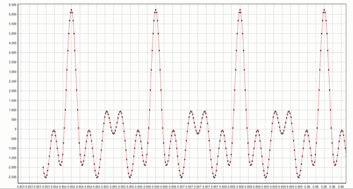
x03 waveform
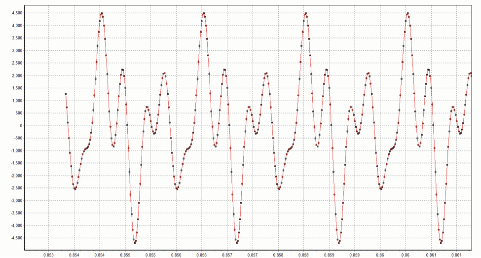
x04 waveform
These graphs demonstrate the first point I wanted to make: dramatically different time domain waveforms can lead to the same audio perception. Perhaps this is really not so surprising — after all, files compressed with the MP3 and AAC algorithms are commonplace. Abstractly, these algorithms can be viewed as techniques for mapping M bits onto N bits where N < M. For algorithms such as these that achieve significant compression, N is much less than M, and the mapping distorts the waveform (we, therefore, say these algorithms are lossy, not lossless). Most of the time we cannot hear the difference between the original and compressed waveforms. Nevertheless, I think it is humbling and important to keep in mind that the ear can be easily fooled into thinking that two distinctly different time-domain waveforms are “identical” when in fact they are not.
How about the case where phase distortions are applied to real music as opposed to the synthetically-generated periodic waveform above? Consider the spock_m.wav file introduced in post 1. What happens if we set the phase of every transform coefficient to zero? It sounds like this: spock_phase0.wav. A graph of the same spot in the two waveforms is shown below (spock_m.wav is in red):
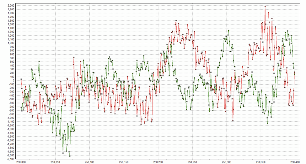
Spock_m in green, Spock_phase0 in red
In this case there is no denying that you can hear the difference between the waveforms, even though they have identical spectrograms! Recall that this was the second point I set out to make. (In terms of simply recognizing what you are hearing, however, I’m sure you had no difficulty in identifying spock_phase0.wav as the Spock clip, even though it sounds different than spock_m.wav.)
How about if we randomly change the phase of every coefficient in every DFT block by using a random number generator to generate a phase value between -π and π for each coefficient? Doing so we obtain spock_phase_ran.wav. This clip is surprisingly easy to recognize, even if Spock does sound like he’s suffering from some weird space sickness. The original and distorted time domain waveforms are shown below for the same spot as graphed above.
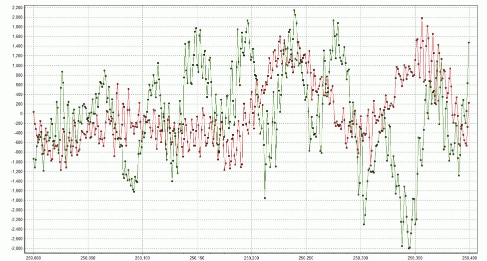
Spock_m in green, Spock_phase_ran in red
Finally, just in case you are a Sherlock Holmes fan, here are the corresponding two waveforms for that theme song: holmes_phase0.wav, holmes_phase_ran.wav.