The web is filled with introductions to
Delta Sigma modulation (also sometimes referred to as Sigma Delta modulation) in the context of Delta Sigma converters. Unfortunately, the ones I’ve looked at fail to intuitively motivate how the modulator works. Therefore, my goal in this post is to show how the structure of a first-order ΔΣ modulator can be simply understood. In particular, I show how its structure can be derived from a trivial 10-line C program that performs the ΔΣ modulator function.
The basic problem solved by a ΔΣ modulator is this: given a fixed input value ν that lies in the range [-1, 1], the modulator outputs a pulse train satisfying the following criteria:
- Each pulse has the same fixed width τ
- Each pulse has an amplitude of -1 or 1 only
- The time average value of the pulse train emitted converges to ν
To derive from first principles a system diagram to perform this task, I find it useful to proceed as follows: First, write down a few equations to make precise what we’re after; next, write a computer program that emits a pulse train satisfying the equations; and finally, draw a block diagram that realizes the computer program.
So let’s get started. First, a waveform f(t) has an average value on the interval of
\mu (T) = \dfrac{1}{T}\displaystyle\int_{0}^{T}f(t)dt
Let l(i) be the magnitude of the pulse of duration t emitted in the interval ; l(i) must be 1 or -1. The average value of the pulse train waveform f(t) corresponding to a sequence of ?pulses is given by
\mu (N\tau) = \dfrac{1}{N\tau}\displaystyle\int_{0}^{N\tau}f(t)dt = \dfrac{1}{N\tau}\displaystyle\sum_{t=0}^{N-1}l(i)\tau = \dfrac{1}{N}\displaystyle\sum_{t=0}^{N-1}l(i)=\dfrac{S(N)}{N}
So we don’t need to worry about τ, which is nice! Here we have defined S(N) to be the sum of the l(i) values from 0 to N – 1, so S(1) = l(0), S(2) = l(0) + l(1), and so on.
How can we write a computer program to decide whether the next pulse to output should be a 1 or a -1? I think the first algorithm most of us would think of is the following: “keep track of the average value, S(N) / N, at each instant. If the current average is less than ν, output a 1 next; otherwise output a -1.” I will skip a formal proof that the pulse train emitted by this algorithm converges as desired, but it is intuitively reasonable that it does, because each additional output pulse moves the average up or down by a smaller amount than the previously emitted pulse, and each pulse nudges the average in the desired direction.
It’s straightforward to write a computer program that accomplishes the above. In C-like pseudo code the program looks like this:
N=1;
while (1) { S_N = compute_current_S_N();
if ( (S_N/N) < v )
output(1);
else
output(-1);
N++;
}
This can be equivalently written as
N=1;
while (1) { S_N = compute_current_S_N();
if( N*v – S_N > 0 )
output(1);
else
output(-1);
N++;
}
Now it’s time to draw a system diagram to implement this algorithm. Clearly, it will contain some sort of feedback because the pulse value to output next depends on the past sequence of output values. There will also be a need to compute a difference, and somehow we will need to accumulate the values S(N) and Nν. Consider the system diagram below:
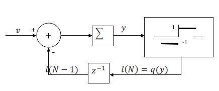
Let’s analyze this diagram to see if it does the right thing. I’ve labeled the input ν and the feedback line l. With respect to the feedback line, the box with a z in it means “delay by one time instant”; the indexes of l on either side of this box reflect that delay. The box with a plus sign in it is an instantaneous summer, which has been configured in this case to take the difference between its two inputs. The large box is a quantizer, and the graph within it shows the input/output transfer function q( ). The graph means that any input value greater than 0 will result in an output value of 1, while any input value less than 0 will result in an output value of -1. Finally, the box with a capital sigma (Σ) in it is an accumulator, also known as an integrator. Its output is the sum of all its previous inputs.
To see if this system diagram results in the required stream of pulses l(i), we need to analyze the variable y. This is most easily done by creating a table as shown below:
| N | l(N-1) | y(N) | l(N) |
| 0 | N/A | y(0) is initialized to 0 | l(0) is initialized to 1 |
| 1 | l(0) = 1 | y(1) = ν-l(0) | l(1)=q( y(1) ) |
| 2 | l(1) | y(2) = (ν-l(0)) + (ν-l(1)) = 2ν – l(0) – l(1) | l(2) = q( y(2) ) |
| 3 | l(2) | y(3) = 3ν – l(0) – l(1) – l(2) = 3ν – S(3) | l(3) = q( y(3) ) |
| …and in the general case | |||
| N | l(N-1) | y(N) = Nν – S(N) | l(N) = q( y(N) ) |
The quantizer is executing the “if then” portion of the computer program, and the summer and accumulator are computing the running sum needed as the argument for the if function (i.e., as the input to the quantizer). This system will do the trick!
This diagram is often written in a slightly different form to more closely model its realization in hardware as follows:
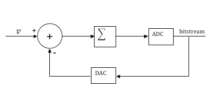
All that is going on here is that the quantizer in the first diagram is replaced with the combination of an analog-to-digital converter (ADC) and a digital-to-analog converter (DAC). The ADC outputs a 1 if its input is greater than 0 and a 0 if its input is less than zero, so a bitstream is created at the indicated point. The DAC converts the bitstream back to a sequence of -1 and 1 values. Finally, to indicate the analog nature of this modulator when used as part of a ΔΣ converter, the accumulator is replaced by an integrator:

Now, assume the ΔΣ modulator above is used as part of an analog-to-digital converter. If the input signal changes slowly relative to the rate at which bits are produced, then many bits will be generated before the signal changes significantly, and the average value the bits encode will be close to the true value. In other words, the 1s and -1s the bitstream represents have time to “average out” to an accurate representation of the input signal. Of course, this average still has to be computed numerically after the modulator; more on that later. However, the faster the input signal changes, the fewer bits will be generated before the signal has changed significantly, and the less accurately the bitstream will represent the signal. At an intuitive level, this is why the quantization noise of ΔΣ converters increases as a function of the input frequency of the signal.
When used as part of an analog-to-digital converter, the modulator is followed by a digital filter and a decimator. The digital filter computes the averages encoded in the bitstream; the decimator reduces the sample rate from the high rate of the 1-bit ADC to the Nyquist rate associated with the final multi-bit samples. The binary representation of the decimated samples is used as the AD output bits.
Part II discusses filtering and decimation in greater detail and presents some simulation results.
Mike Perkins, Ph.D., is a managing partner of Cardinal Peak and an expert in algorithm development for video and signal processing applications.