R₀ and COVID-19: A Simple DSP Perspective

Cardinal Peak knows nothing about COVID-19 and epidemiology, but as a DSP or digital signal processing company, we do know a thing or two. For those interested in viewing disease spread through that lens, this blog presents — and solves using Z-transforms — a trivial difference equation incorporating the much-touted variable R₀.

1. The Model

Let R₀ be the average number of people each person who contracts the disease will subsequently infect. To keep things simple, we’ll assume that the susceptible population is enormous so that the disease can spread unimpeded for a significant time. In other words, herd immunity is far in the future! We’ll also assume that everyone who gets infected at time n infects R₀ people in the very next time interval and never infects anyone else after that. With these assumptions, if we let x(n) be the cumulative number of people infected at time n, we can immediately write the following equation:

x(n)=x(n-1)+R_{0}(x(n-1)-x(n-2))+g(n-1)

In words, this equation says that the total number of people infected at time n depends on three things:

1. The total number of people infected at time n – 1, i.e., x(n – 1).
2. The number of people infected by the people who first became infected at time n – 1. This is the trickiest term to understand. The number of people who were first infected at time n – 1 is given by x(n – 1) – x(n – 2), and we are assuming that each of them infects R₀ new people, so we must multiply those factors together.
3. The number of infected people migrating into the population between times n – 1 and n, which we’ll call g(n – 1). This term may seem superfluous, but it makes dealing with initial conditions easy and facilitates a Z-transform solution.

2. The Solution

The Z-transform of the above difference equation is:

X(z)=z^{-1}X(z)+R_{0} z^{-1}X(z)-R_{0}z^{-2}X(z)+z^{-1}G(z)

This can be solved for X(z) in terms of G(z), yielding:

X(z)=\dfrac{z^{-1}G(z)}{1-(R_{0}+1)z^{-1}+R_{0}z^{-2}}

The simplest initial condition is to assume that the infection starts with a number of people, g₀ , who enter the population at time n = 0. Example: a group of infected people from a cruise ship disembark in a port where the virus doesn’t yet exist. We’ll assume no other infected people migrate into the population after that initial event. The corresponding Z-transform, G(z), of g(n) = {…,0 ,0 ,0 ,g₀ , 0, 0, 0, …} is just g₀. We therefore have:

X(z)=\dfrac{z^{-1}g_{0}}{1-(R_{0}+1)z^{-1}+R_{0}z^{-2}}

You can look up the solution for x(n) in a table of Z-transforms (we’re engineers after all). Or, if you’re a purist, you can use the quadratic equation to find the roots of the denominator (they’re 1 and 1/R₀), use the method of partial fractions to express X(z) as a sum of two terms, and then use algebra and the fundamental Z-transform relationship.

a^{n} \longleftrightarrow \dfrac{1}{1-z^{-1}a}

Either way, you’ll find that the solution is:

x(n)=\dfrac{g_{0}}{1-R_{0}}(1-R_{0}^{n})

The only problem with this solution occurs when R₀ = 1 because the (1 – R₀) in the denominator becomes zero. In this special case, using L’Hopital’s rule yields:

x(n)=ng_{0}

3. Discussion

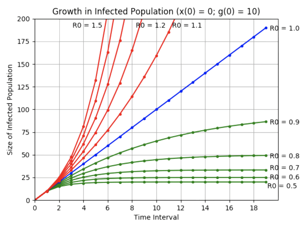
When R₀ = 1, the number of people infected grows linearly. This makes intuitive sense; each infected person infects exactly one more person. Eventually, the disease will spread through the entire population. On the other hand, when R₀ < 1, the number of infected people will asymptotically approach g₀ / (1 – R₀). Finally, when R₀ > 1, the size of the infected population will grow exponentially. The graph below illustrates a few cases.

For completeness, let’s draw the connection of our difference equation approach to the sum of a geometric sequence. If we start with g₀ infected people at time 0, each of them will infect R₀ new people, so an additional g₀R₀ people will be infected by time 1. Each of these newly infected people will, in turn, infect R₀ susceptible people, leading to an additional g₀R₀² infections by time 2. Continuing this line of reasoning, at time n, the total number of infected people is given by:

x(n)=\displaystyle\sum_{k=0}^{n-1}g_{0}R_{0}^{k}

The formula for the sum of a geometric sequence is also easy to look up, and it will give the same result we derived above by starting with a difference equation.

To discover how we help teams use signal processing to achieve the highest level of product performance, check out our Signal Processing expertise page.