In the first post of this three-part series, I listed four points that I hope my readers will agree with at the end of this series. The second post addressed the first two points of the four. In this post, Part Three of the series, I will demonstrate the final two points:
- Phase distortions generally have less effect on human perception than magnitude distortions; and
- Two audio clips can be recognized by humans as matching despite having dramatically different spectrograms.
In Part One I explained the concept of a spectrogram and how it is computed using the DFT. In Part Two we looked at the effect of distortions on human aural perception. We found that in some cases phase distortions change the time domain waveform but have no effect on our perception. In other cases, phase distortions clearly affect the audio, but the distortions have no impact on our ability to easily recognize a clip. In this final part, we will look at the effect of spectral magnitude distortions. Unlike the case with phase distortions, magnitude distortions change the spectrogram.
Let’s begin with the clip x03.wav first introduced in Part One. Recall that it is a sum of five sinusoids, with frequencies of the five sinusoids, in Hz, are {500 Hz, 1000 Hz, 1500 Hz, 2000 Hz, 2500 Hz}. The magnitudes of the five sinusoids are {1000, 2000, 750, 1000, 1500}. The waveform x03.wav was formed from the following sum:
x03(n)=\displaystyle\sum_{l=1}^{5}a_{l}\cos(2 \pi f_{l}nT+\theta_{l})
where the sampling rate is 48 kHz (T=1/48,000) and the five phase values f are {0, 0, 0, 0, 0}. What happens if we change the magnitude values to the five randomly chosen values {427, 716, 2113, 1382, 373}? The result is the file x05.wav. Waveforms for both x03.wav and x05.wav are shown below:
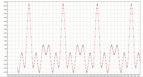
x03 waveform
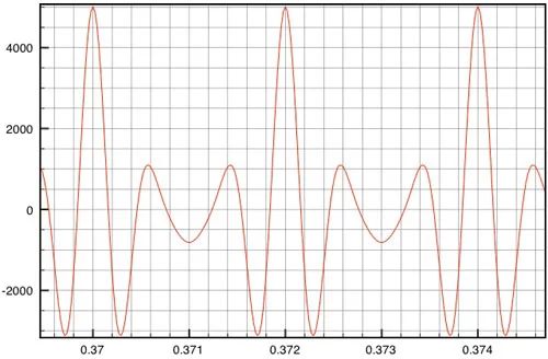
x05 waveform
The spectrograms of these two waveforms appear below (x03.wav is on top). The frequencies are the same, although the 2500 Hz sine wave is barely visible in x05.wav because its magnitude is so small. It is clear that the intensities for each frequency in x05.wav are different from those in x03.wav; in other words, the spectrogram has changed.
![]()
![]()
If you listen to these two clips you’ll hear that it is easy to tell them apart. Note how different this is from the case examined in Part Two where a random change of the sinusoids’ phases led to a waveform that sounded the same, although its time domain graph showed it was different. This is an illustration of the fact that the ear is generally less sensitive to phase distortions than to magnitude distortions. Furthermore, if you compare x05.wav’s waveform above to that of x04.wav in Part Two I think you’ll agree that it is hard to look at two time domain waveforms and know in advance whether they will sound the same, or different, as a reference waveform (in this case, x03.wav).
In Part Two we did the experiment of keeping the magnitudes for the Spock clip the same while assigning random phases to the DFT coefficients. This does not change the spectrogram. What if we assign random magnitudes to the DFT coefficients while keeping the phases the same? This DOES change the spectrogram. Below are pictures of the spectrograms in these two cases; the corresponding audio files can be found in spock_ran_mag.wav and spock_m.wav.
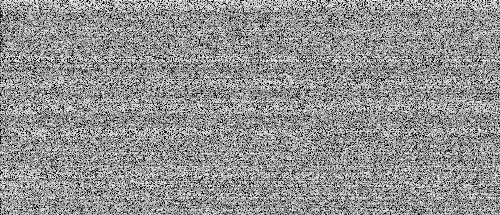
spock_ran_mag spectrogram
spock_m spectrogram
If you listen to these clips you’ll see that it is impossible to recognize the magnitude-distorted clip as Spock. This too illustrates that the ear is more sensitive to magnitude distortions than phase distortions.
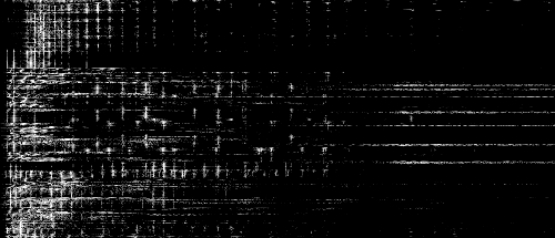
Now we want to consider a case where the Spock spectrogram is dramatically different, yet the clip is still easily recognizable. Consider the following processing: for each row of the spectrogram, find the maximum magnitude of a DFT coefficient. Then, for all coefficients in that row, if the magnitude of a DFT coefficient is within 40dB of the maximum, set its magnitude equal to that of the maximum (keep the phase the same), otherwise set its magnitude to zero. This processing results in a spectrogram with only two levels: on or off. A given frequency is either present or not. The processing throws away coefficients that aren’t carrying much energy (they are more than 40dB down from the maximum). The spectrogram looks like this:
spock_2level spectrogram
I think you’ll agree that this is substantially different than the spectrograph of the original clip. Nevertheless, you will have no trouble identifying the clip if you listen to it: spock_2level.wav. This example demonstrates the final point I set out to show: that two clips can be recognized as the same even if they have dramatically different spectrographs. As an even more amazing demonstration of this, what if we set every DFT coefficient to the same magnitude while preserving its phase. The spectrogram is now solid white — every frequency is present with the same magnitude throughout the entire clip. Amazingly, the clip can still be identified (especially when Spock is speaking): spock_cnst.wav. This demonstrates that although the magnitude may be more important for aural perception than phase, the phase alone carries enough information, albeit just barely, to recognize a clip.